This is part 7 of a series of 8 articles from the European Institute for Climate and Energy, translated by Google (so please excuse the quality or lack thereof).
Click here for the original article.
Part 7: Dynamic Solar System - the actual effects of climate change. The influence of the sun on the cloud cover beyond Svensmark
As has long been known, the cosmic rays, whose impact on the Earth is determined by the Sun's activity, are a significant influence on the lower cloud cover and thus on our
weather/climate - Svensmark effect. CERN had recently confirmed for the first time this influence in the lab, and thus awarded the Svensmark effect to be correct. In all temperature
models, this effect on the cloud cover, which is significant for our wether and thus the climate, has not been unaccounted for.
For this reason alone all the climate scenarios of the IPCC are wrong.
Not without a reason, the legwork-people of the IPCC, such as PIK, have worked hard in recent years to deny this indirect influence of the sun and to show that it does not exist.
Well, with the results of CERN, the discussion is on a different level. It is now no longer about "if" but about "how much".
Beyond the known Svensmark effect, there are additonal direct influence of the sun on the cloud cover and thus on climate and extreme weather events such as hurricane and tornado
activity. This is the content of Part 7.
The influence of the sun on the cloud cover beyond Svensmark
The influence of cosmic radiation on the temperature are shown in Figures 148 and 149, Source: Science, Vol 309, pp. 2017-2024, 23 September 2005. The consistency of the
smoothed curves is striking.
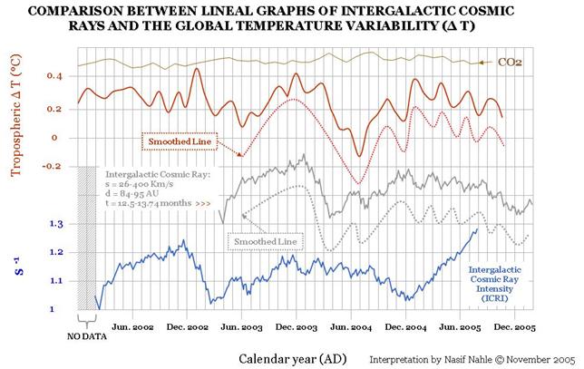
Figure 159: The figure shows also no correlation with the temperature of the CO2 curve, however, a clear compliance with the temperature of the cosmic radiation.
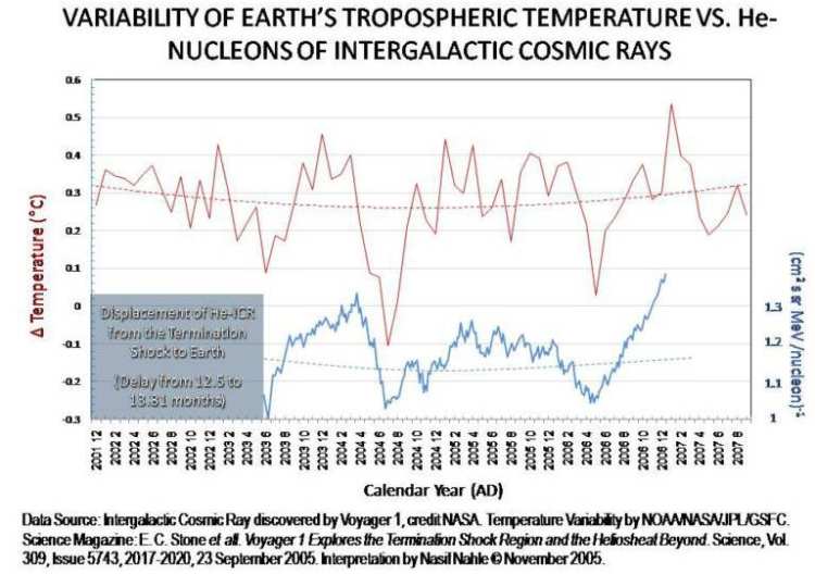
Figure 160 shows the temperature curve (DT) of the lower troposphere to the cosmic radiation from December 2001 to August 2006. It can clearly be seen that not only the smoothed long-term
trend (dotted line), but also the minima and maxima match. The figure was added on 21 October 2007 to the first-mentioned figure.
At the beginning, the effect should be outlined, via which the sun directly influences the earth's atmosphere and thus changes the state in the atmosphere, which exerts a direct
influence on weather and climate. The crucial role have the electric charged aerosol particles in the atmosphere, which will be moderated directly by HCS (Heliospheric current sheet) and
solar wind.
By cosmic radiation, air molecules are ionized, ie electrically loaded. With sulfur dioxide, which is located in the atmosphere, ionized sulfuric acid is built in several chemical steps.
Together with "normal" sulfuric acid and water molecules it creates cluster ions. The charge (negative) of the cluster relieved (by a factor of 10) the addition of other neutral molecules.
Thus a so-called critical cluster can be formed. Tthe addition of further molecules results in an Aerosol particle. Above a certain size (100 nm), a condensation nucleus for the
droplet generation forms.
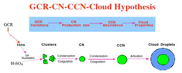
Figure 161 Source: Fangqun Yu, Atmospheric Sciences Research Center, State University of New York "Cosmic rays, particle formation, natural variability", shows the beginning of the
cloud formation process. It is known that sulfur aerosols, particularly sulfuric acid, influences temperature, pressure and density in the layers of the atmosphere. Additionally is a further
parameter, the ion density. Caused by for example cosmic radiation, ions, electrically charged atoms, result which for example form sulfuric acid, present in the atmosphere, together to
clusters. These clusters are the basis for condensation nuclei (CN = condensation nuclei). An increase of nanoparticles causes the increase of the cloud condensation nuclei
(CCN cloud condensation nuclei), because water vapor may bind well to this. This results in small water droplets (cloud droplets).
Next, it is known since the inventor of the fog chamber, Charles Thomson Rees Wilson, that ions of oxygen molecules are immediately surrounded by water droplets. In the lower
atmosphere, these are the nuclei for raindrops.
Surface and the atmosphere have different electric potentials. Therefore, there is an ongoing potential gradient. The data in the literature vary between 250 kV and 500 kV. There is
therefore a plurality and free charges in the atmosphere. The most famous charge balance is held by lightning.
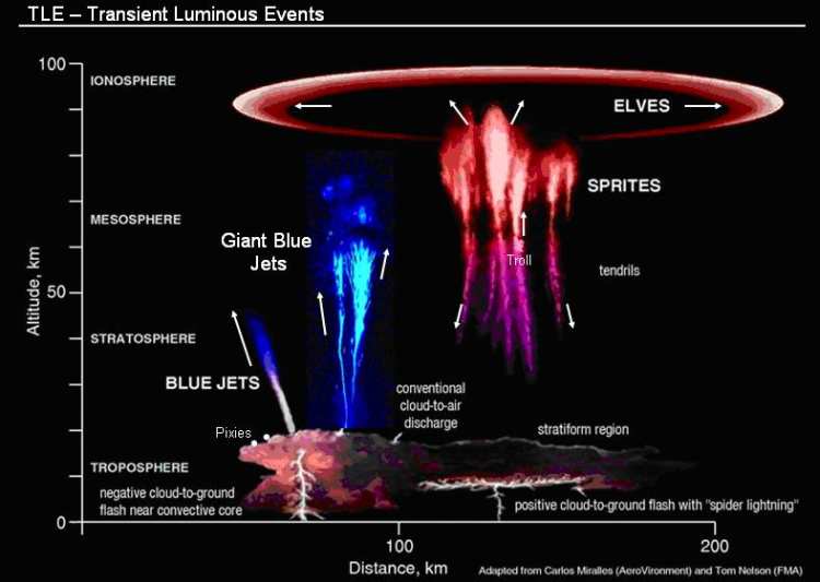
Figure 162: Electrical discharges in the lower troposphere, like lightning, or in the Stratos and mesosphere in the form of blue jets and red sprites, are just the visible manifestations of
electricity in the atmosphere. Thus it can ever happen, there must be free electric charges, and their local concentration generate visible leakage currents, source: "Red sprites and
blue jets," Jens Oberheide, University of Wuppertal.
The ionization in the upper atmosphere (ionosphere, an electrically conductive layer) is formed by the absorption of UV radiation from the sun through the air molecules and atoms
in the ionosphere. Due to the ejection of electrons by the high-energy UV radiation a positive potential shift is induced. Technically this is called "leveling course", which faces the
negative potential shift, the ground. Earth and ionosphere, both good electrical conducting, act as a spherical capacitor with a dielectric, the atmosphere between them.
In this dielectric a constant potential flow takes place, which is characterized by the space charge and the charge transport. This potential flow is called "Global Electrical Circuit",
see the following illustrations.
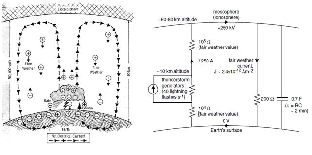
Figure 163 left, source: (http://www.meteo.psu.edu/~verlinde/meteo437/figures437.html) shows the global electrical circuit in the atmosphere and the ground. The figure on the right, the
electrical equivalent circuit diagram, source: ( http://www.slac.stanford.edu/cgi-wrap/getdoc/slac-wp-020-ch11g-Kirkby.pdf ).
The illustrated electric field is usually directed downwards. Only in bad weather (eg thunderstorms), the field is directed upward. The field strength is close to the ground about 150 V/m
and decreases rapidly with height. From balloon measurements, its field strength in 10-km height is only 5 V/m. The decrease in field strength can only be due to the fact that there
are space charges in the atmosphere that are parallel to the field. The resulting field is the measure of the field strength.
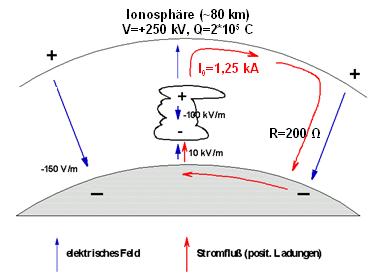
Figure 164: As with a voltage applied across a capacitor, a directed compensating current is flowing between the ionosphere and the ground, the "vertical flow". He is small and has good
weather field values of some pico A/m2, which rise in bad weather conditions at orders of magnitude and are of short duration. According to the Institute of Atmospheric Physics of the University of
Wuppertal, the total current is from thunderstorms at 1,250 amps. Over longer time scales, the electricity is balanced, so there can not be a charging, for example of the ground.
What other processes such as the high-energy ultraviolet radiation from the sun result in charge carriers (ions, electrons) in the atmosphere? These are, as already mentioned, the
cosmic radiation, which ionizes air molecules in the Stratos- and troposphere and these are turbulence in atmospheric layers (eg, thunderstorm clouds), which are released electron by collisions.
In addition, Prof. Galembeck (University of Campinas, Brazil) found that moist air electric charges when it anneals adsorb to dust particles (aerosols) in the atmosphere. The water in
the atmosphere is electrically charged through this process, positive or negative, depending on dust particles. The researchers call this process Hygro electricity.
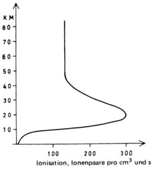
In summary, it can be stated that in the atmosphere caused by different processes constantly electrical charge carriers accrue, which as of electric charged aerosol particles affect the
cloud cover and weather conditions. Electric charged aerosol particles as a constellation of germs are up to 10 times more effective than uncharged. As figure 165 (above) shows, Source:
General Meteorology (3rd edition), Gösta H. Liljequist, Konrad Cehak, arise especially in the lower stratosphere and upper troposphere by cosmic radiation ion pairs. Upper troposphere
and lower stratosphere is the altitude range where the Jet Stream influence significantly the atmospheric weather conditions in the northern hemisphere. It is therefore
not so far off that a modulation of the electrical particles in the atmosphere influence by direct or indirect solar influences, both the atmospheric weather conditions (jet), as well as the local weather
conditions (cloud cover).
This increase in the areas of the jet stream all the more so because not only the ion density increases sharply, but because of the lower pressure (lower probability of collision), the ion
mobility, and thereby determined also their life span is increased. These electrically charged particles can basically be influenced by an external potential field or an applied current.
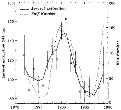
As Figure 166, Source: V.C. Roldugin and G.V. Starkov , " Dependence of Atmospheric Transparency Variations on Solar Activity "( Polar Geophysical Institute, Apatity, Russia) documents,
there is a clear correlation between the sunspot number (Wolf number) and the aerosol attenuation (index) in the wavelength range between 344-369 nm.
The aerosol formation varies directly with the solar activity. The stronger the solar activity, the more the aerosol formation declines.
This work conforms to the Svensmark effect, which calls, that the cloud cover increases through increased cosmic radiation, because the ion formation rate and thus
the number of condensation nuclei for raindrops increases.
The electrical conductivity of the atmosphere, as well as the number of flashes varies with the cosmic radiation, Figure 167, Source:
( http://www.slac.stanford.edu/cgi-wrap/getdoc/slac-wp-020-ch11g-Kirkby. pdf ).
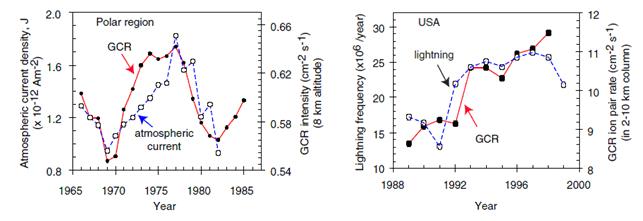
Figure 167,left, shows the fluctuations of the vertical current to the cosmic radiation (GCR) in the polar region and the right figure, the flash frequency per year depending on the
GCR in the United States. Both the vertical flow, and the flash frequency varies with the cosmic radiation.
How much electrical effects in the atmosphere control the condensation and thus the amount of rain is visible at a Forbush event (after the geophysicist Scott E. Forbush,
who discovered the effect). A Forbush event is a sudden drop in the cosmic radiation due to sudden strong solar activity, because of increased solar activity the solar wind
deflects cosmic rays from the earth. In an SCR event ( S olar C osmic R ay) high-energy protons from the sun reach to Earth.
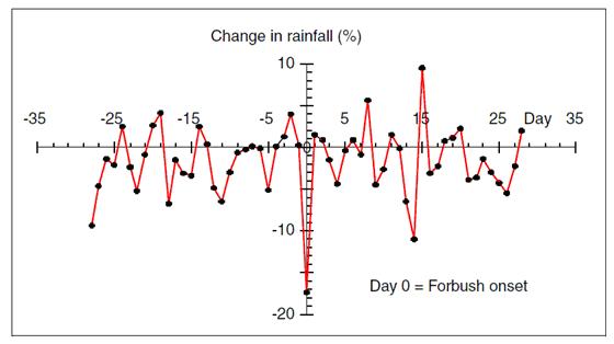
Figure 168 shows the decline in rainfall during a Forbush event (During Forbush decrease GCR) . It clearly shows that the rainfall is declining sharply, which is due to the fact that less
electrically charged aerosols for rain drops are available. Source: http://www.slac.stanford.edu/cgi-wrap/getdoc/slac-wp-020-ch11g-Kirkby.pdf
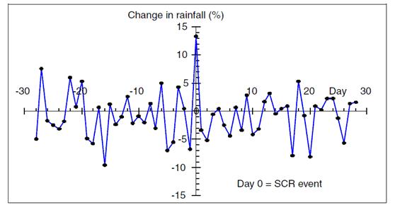
Figure 169 shows the change of rainfall during an SCR event (During ground-level, SCR increase, source as above). It is found that the amount of rain increases significantly,
due to the increasing ionization in the atmosphere and in an increase of electrically charged aerosol particles.
The presented studies support, that a variety of electrically charged aerosols are available in the atmosphere, and that water in the atmosphere is electrically charged and the weather is
influenced by changing of the electrical parameters in the atmosphere. The influence can never come from CO2 - for this there is no physical basis - but only by the sun.
From the following figure it's evident how the solar activity (using the example of the aa-index) changes the air pressure in the atmosphere in the tropics generally.
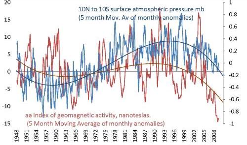
Figure 170 Source: (http://climatechange1.wordpress.com/2009/11/08/the-climate-engine/) shows the variation of the aa-index in the period from 1948 - 2009 (red) and to that
the fluctuations of the surface air pressure in the tropics (blue). It is clearly apparent that both are related, the solar activity moderates the air pressure in the tropics and thus the
weather - air pressure differences are known to drive the weather. The smoothed trend corresponds to the Gleissberg cycle.
Figure 171 shows how the aa-index is determined by solar activity, the Schwabe cycle and the increase of the de Vries-Suess cycle in the 20th Century.
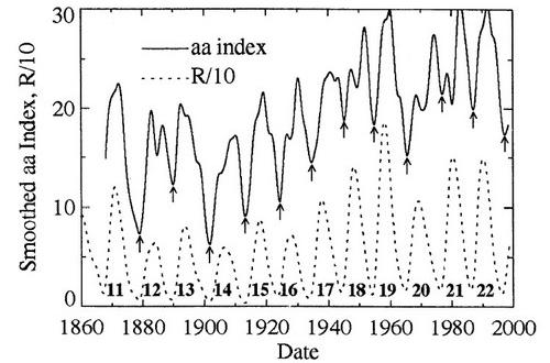
Figure 171, Source: Hathaway, et al. 1999" A synthesis of solar cycle prediction techniques, Journal of Geophysical Research, 104 (A10), 22375-22388 DOI: 10.1029/1999JA900313
shows the aa-index and the Schwabe cycle (dotted line). It is clearly shown in the aa-index. In the 20th century it increases dramatically parallel with the de Vries/Suess cycle.
To which extent the magnetic activity of the Sun and the polarity of the solar magnetic field control the parameters of the terrestrial weather system is shown in figure 172, which
shows the cloud cover according to data of the International Satellite Cloud Climatology Project shows (ISCCP).
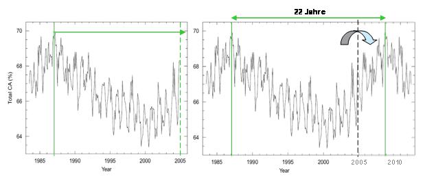
Figure 172, left, shows the global cloud cover from July 1983 - June 2005, according to data from the ISCCP, (http://www.leif.org/research/cloud-cover.png). The image comes from the
work of Evan et al. "Arguments against a physical long-term trend in global ISCCP cloud Amounts." The left-hand image already shows a periodic oscillation of greater than 18 years
(green arrow). The minimum curve is in the maximum of the 23. Schwabe cycle in the year 2000. Right is the curve mirrored on the dotted line and set from 2005.
It was ensured that the relationship
between growth and decline in the Schwabe cycle is about 2 to 3 (the rise time is not exactly fix, but depends strongly on how strong the next cycle is - strong cycle = fast rise time,
low-cycle = slow Rise time, so far the ratio 2 to 3 represents an average). The maximum of the global cloud cover depends in a unique way on the Hale cycle (polarity cycle of the sun)
and thus on the polarity of the magnetic solar cycle.
Now, of course, it can be argued that the above reflection are not actually measured values, from which the cycle time could be derived. In fact, the measurements until 2008
(then the project IPCCP was closed and additional data are not available to the author) show that the cloud evolution from 2005 does not rise again, but remains low.
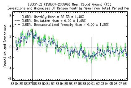
Figure 173 ( isccp.giss.nasa.gov/climanal1.html ) shows the entire data set of the global cloud cover by 2008. While the cloud cover from its minimum in 2000 is rising again to 2004, it then
stays at this level and does not increase further. At the black vertical lines the trend of cloud cover in each case turns, it is consistent with the rotation of the polar field of the Sun (Figure 174).
How does this fit the Hale cycle of 22 years, which is known as a vibration with a period of about 22 years and not a decayed state, in which the values remain the
same and do not change over the years? The answer is found in the solar activity of the Schwabe cycle, which is known to be a part (half) of it.
Two Schwabe cycles, result in a Halezycle, because then the polarity of the magnetic fields of the northern and southern sunspot is again the same. As a reminder, with a new
Schwabe cycle, the magnetic polarity changes on the respective hemisphere.
The 23. Schwabe cycle was -as is well known- with a duration of 14 years significantly longer than the average of 11 years. Whereas his rise time until reaching its maximum of 4-5 years
was within its predecessor's, his drop, until the beginning of the new solar cycle was with 9 years exceptionally long, as Figure 174 shows on the left.
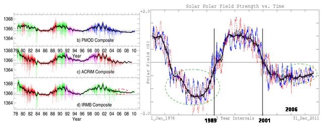
Figure 174, left, shows the last three solar cycles until 2010. The 23. Cycle lasted much longer than its predecessor and its minimum lasted for several years, with only very little changed
solar activity. These are the years 2006 - 2009 (red circle). The illustration to the right, source: Wilcox Solar Observatory, Stanford University (http://wso.stanford.edu/) shows the polar
magnetic field of the sun until 2010. The polar magnetic field of the sun, which dominates in the solar minimum, and dictates the polarity (dipole) of the solar magnetic field, is highly stable
since about 2005, and also shows a "decayed" state (right circle), whereas in the previous graph minimum, this is only briefly and directly passes on to its oscillation state (left circle).
It should be noted therefore that
-
also the ISCCP cloud coverage after 2005 reflects accurately the solar activity, which is determined by the Schwabe cycle
-
the 3 years of sustained, steady and not changing low cloud cover matches with the long, tapered 23rd Schwabe cycle, which is also not changed and out of it (Polar box, right green circle)
-
during this period no polarity reversal took place, which would might have changed the degree of coverage
-
a polarity reversal failed up to this time - on the contrary, the polarity in the same period over the same period as the cloud cover fluctuates around a mean value.
-
with a zero crossing of the polar field (polarity reversal, black, vertical lines) rotates the cloud cover grade. This was around 1988/89 and then again around 2001.
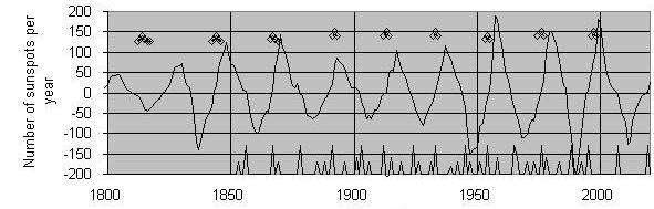
Figure 175 shows the Hale cycle ( http://nexialinstitute.com/climate_el_nino.htm) of 1800 - 2009 (upper data set). The rhombs indicate U.S. dry years and the lower data set
shows El Niño events.
Whereas El Niño-events do not indicate a direct relation to the Hale cycle (it was shown in detail in part 1 how El Niño is controlled by the sun) the U.S. dry years, so clouds
weak years, show a marked accumulation to the Hale cycle and that whenever the polarity of the solar magnetic field is N+ and S-. This points to a connection with the formation of aerosol
particles and thus the condensation nuclei for cloud.
From another study, "Does the solar wind affect the solar cycle?" Israelevich et al., Astron. Astrophys. 362, 379-382 (2000), is the following series of the Bz component.
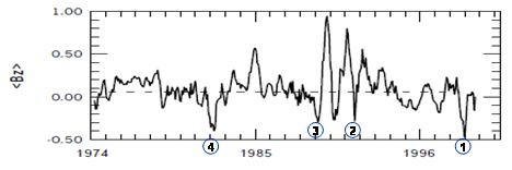
Figure 176 shows the Bz 1973-2000 as a moving average over seven solar rotations. The dashed line shows its mean to the period under consideration. Striking is the strong negative peak
in 1998. Throughout the period, this is the strongest negative component. It coincides with the strongest El Niño event in 50 years. As shown in section 5, the magnetic field is so much weaker
and there are even more northern lights, the more negative the Bz is.
Another indication that the polarity of the IPF affects the cloud cover is found in the evidence of the influence of cosmic radiation on the lower cloud cover.
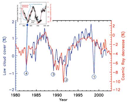
Figure 177 (Source: Marsh and Svensmark, 2003) shows the lower cloud cover (blue) from 1983 to 2002 according to data from the ISCCP and the cosmic radiation measured in the
number of neutrons. It shows the strong correlation of both parameters. The lower cloud cover is subject to the beat of the CR, variations of 2-3%. One can notice the sharp decline in
cloud cover in 1999, which can not be found in the cosmic radiation. It is however clearly seen in the Bz-component (previous figure). The minima 2), 3) and 4) in the Bz are also found in
cloud cover again (Figure 176).
Note to the figure: Since the time series of low cloud cover at Marsh & Svensmark begins not before 1983, the imagery of cloud cover, which time series starts at 1980
(1980 - 1995, small picture), but has a different smoothing, is used for comparison of the minima 4. The minima in the cloud coverage from there in 1982 coincides also with the strong minima of Bz in 1982.
In the small figure, the minima around 1990 is not sharp marked, as in 1982, but flat, suggesting that it originates from multiple triggers. Looking at the Bz,
three minima can be found in the fine-resolution in the period 1990 - 1992 (Figure 176).
HCS and the IPF are the effects of solar activity, which have their origin in the convection zone and the tachocline of the Sun. The middle piece, which so to speak ties together
cause and consequences, is the solar corona, in which accrues the solar wind and with it the IPF and the HCS. Therefore it was necessary to treat this before.
From these findings, it is only a short step to saying that the heliospheric current sheet (HCS) directly affects the cloud cover and thus the weather on the Earth.
The two scientists D.R. Kniveton (University of Sussex) and Professor B.A. Tinsley (University of Texas), "Daily changes in global cloud cover and Earth transits of the Heliospheric current
sheet "(http://www.utdallas.edu/physics/pdf/tin_dcgcc.pdf) went into the question of whether a passage of the earth through the HCS affects the cloud and found the following dependence.
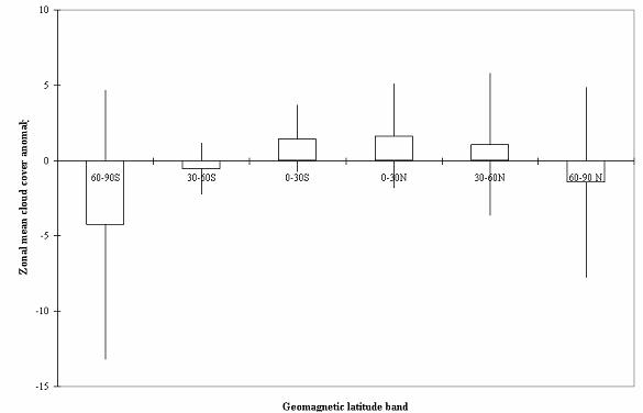
Figure 178 shows the daily changes in the zonal cloud changes during the passage of the earth through the HCS. While at the poles the cloud cover decreases, in the southern
hemisphere even by almost 5%, in the tropics is a recorded increase of 2%. These are values, as at the clouds changes by cosmic rays. Measurements were made in the years
1987 - 1994, ie in the cold phase of the AMO.
The work of Kniveton and Tinsley shows that particularly in the tropics, the cloud cover during passage of the earth through the HCS increases, when the earth atmosphere
is charged with a current of 25,000 amperes. Therefore should be investigated to what extent the HCS has impact to the Atlantic storm development, and in particularon the hurricane activity.
For this purpose the Svalgaard-list of the Wilcox Solar Observatory at Stanford University (http://wso.stanford.edu/SB/SB.Svalgaard.html), which lists the HCS crossings of the earth,
and the ACE list of hurricane Center of NOAA (http://www.nhc.noaa.gov/pastall.shtml) were evaluated.
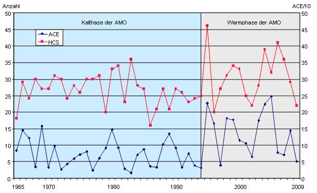
Figure 179 shows the annual number of HCS crossings of the Earth from 1965 to 2009 (red), and the intensity of hurricanes/10 in the same period. The start time was set to 1965,
because from this date the ACE satellite data are available, that have a reliable and consistent character. Before that it was manually counted/measured and the data collected from multiple sources.
Figure 179 indicates that HCS has an effect on hurricane activity. As is known, the North Atlantic hurricane activity is connected to the AMO, the AMM (wind shear) and the
Easterlay-Waves. Figure 180 shows the relationship of hurricane activity with the AMO.
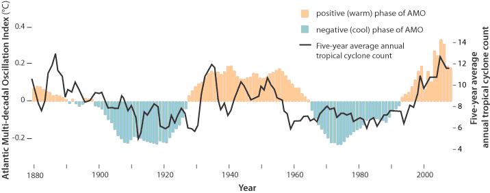
Figure 180 shows that the Atlantic Multi-decadal Oscillation AMO, Source: Landsea et al, 2010, "Impact of Duration Thresholds on Atlantic Tropical Cyclone Counts". Additionally the
course of the tropical hurricanes (black line). AMO and hurricane activity are parallel.
Therefore, it is obvious to mirror the hurricane activity at the HCS plus the AMO, which is also moderated by the sun (figure below). For this purpose, the AMO data from the
NOAA (http://www.esrl.noaa.gov/psd/data/timeseriesimeseries/AMO/) was evaluated and standardized to the lowest value during the observation period, so chosen that as the reference point.
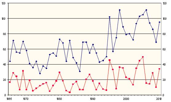
Figure 181 shows the normalized values of the HCS + AMO for the period from 1965 - 2010 (blue curve). To that the ACE in the same period. To facilitate comparisons, the
respectively ACE values were divided by 5, so to see is ACE/5 (red curve). Especially in the warm phase of the AMO, a good correlation of HCS can be seen with the hurricane activity.
The study shows that there is a correlation between HCS-passage and the Atlantic hurricane development. The data series is not as clear as that of the corona on the El Nino events
(part 1). This can not be expected because the hurricane activity depends also on other parameters such as Easterly Waves and wind shear, which are not included in the figure above.
Next, the passages of the earth through the HCS are of course no standard passages. The impact that the HCS has on the Earth's atmosphere is different at each pass. This on the one hand
is related to the Ballerina skirt, i.e the solar activity itself and, secondly, to the respective current distribution in the HCS, which, as shown, is inhomogeneous,
with local maxima and minima. Then the value for the current strength of the HCS is approximately 25,000 amperes, an average which is likely diverging spatially a lot.
Also, the earth partially passes in a passage not only one polarity, but two.
The data series of the HCS to the ACE suggests that the HCS is another parameter that affects hurricane activity in the Atlantic. All the more so as the work on the daily changes in
the zonal cloud cover during earth-passage through the HCS (Kniveton and Tinsley) were conducted in the cold phase of the AMO and at measurements in the AMO warm phase
a higher change value in the zonal cloud cover in the tropics can be expected. This is due to the increase of water vapor in the atmosphere in warmer water.
Especially in the warm phase of the AMO exists a good correlation of hurricane events with the passages of the earth through the HCS.
As a hurricane requires energy for its formation and the
amount of energy in warm AMO is higher, the HCS can so to speak preferred help to trigger a hurricane. The trigger requires warm water temperatures and thus the warm phase
of AMO favors the hurricane activity. In cold surface water (cold phase of the AMO), the zonal cloud cover increases in the tropics during the passage of the earth through the HCS.
Due to the relatively low water temperatures, the low-pressure area lacks energy, respectively energy difference between water and the upper troposphere, which is required in order to grow
into a hurricane.
Finally, it should be noted that the coupling of the cosmic radiation, the Hale cycle and the HCS on the charged aerosol particles in the tropo-and stratospheric significantly influences
the weather/climate.
Not only that hurricane activity is controlled by the sun, but also the tornado activity in the United States.
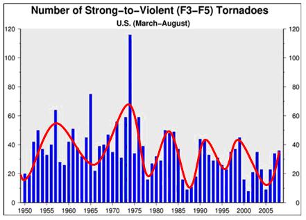
Figure 182 shows the number of severe tornadoes in the United States from 1950 - 2008. The highest number occurs precisely in times of cooler temperatures in the northern
hemisphere in 1960ies and 1970ies. This is due to the large temperature contrasts between the tropics and polar regions, leading to higher wind speeds (Jetstream - tornadoes
and storms/hurricanes in Central Europe are directly related to the occurrence, course and intensity of the jet stream). When solar radiation is reduced by the tilt of the Earth's axis
the relative energy change in the tropics is lower than in the northern hemisphere, resulting in a larger pressure gradient (stroke is greater). The chart shows an average 11-year wave
pattern (red line in 1950 - 2005 = 5 cycles) which coincides with the Schwabe cycle of the sun. If the vibration continues, the next peak of the severe tornado activity falls to
the year 2011, as we experienced this year.
Part 1: The sun sets the temperature response
Part 2: The sun - the amazing star
Part 3: Sunspots and their causes
Part 4a: The atmosphere of the sun: The corona
Part 4b: Heliospheric current sheet and interplanetary magnetic field
Part 5: The atmosphere of the sun: The corona
Part 6: The influence of the sun on our weather / climate
Part 7: The influence of the sun on the cloud cover beyond Svensmark
Part 8: Future Development and the temperature fluctuations
|
|
|