This is part 4b of a series of 8 articles from the European Institute for Climate and Energy, translated by Google (so please excuse the quality or lack thereof).
Click here for the original article.
Part 4b: Dynamic Solar System - the actual effects of climate change. Heliospheric current sheet and interplanetary magnetic field
Heliospheric current sheet (Heliopheric Current Sheet) and interplanetary magnetic field reach far beyond the boundaries of Earth's orbit and thus determine significantly the weather
patterns on Earth, such as CERN confirmed. Both are the link partner of the variable Sun to the Earth. Enter the variable sun, so to speak to our front door and into it thus in our weather
and climate events. Since the postulates of Svensmark that cosmic radiation significantly affected the cloud cover on ionizing particles (nucleation) and the recent confirmation by the
CERN, the electrical processes in the atmosphere, which usually are only electrical discharges, i.e. flashes, but which are much more complex, have special importance. The
continuation of Part 4 shows solar parameters that have the potential to take here effect in the same way as the cosmic radiation.
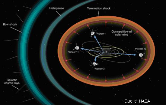
Figure 91 shows the extent of the heliosphere up to the limits of the solar system at about 22.5 billion km.
Heliospheric Current Sheet (HCS)
Since the interplanetary magnetic field on the Earth's orbit is with up to 1 - 10 nT, 100 to 1000 times stronger than the dipole field of the sun promises (magnetic
dipole fields decays with the cube of the distance), there must be an effect, that amplifies this. This is the Heliospheric current sheet that extends to the limits of the solar wind.
She has a width of about 60,000 km (table http://wind.nasa.gov/mfi/hcs.html #). The electrical current in the HCS is directed radially inward and is about 10^ -4 A /km^2. Contrary
to the sun's rays, he does not opertate in the circle, but on the spherical surface of the earth, if the earth pass it. With a diameter of 12,800 km (with atmosphere) an area current of 25,000
amperes and more can impact on the half of the earth's atmosphere.
The Sun rotates differentially on its axis, which is 7.2° inclined to the ecliptic. At the sun-equator is the orbital period about 25 days, at the poles 36 days (in the convection zone
of the Sun, the orbital period is 27 days).
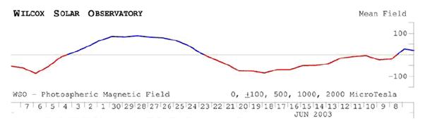
Figure 92, source (www.sotere.uni-osnabrueck.de/spacebook/spacebook_files/lectures_d/space-kap6.pdf) shows the so-called Carrington rotation of the sun with an average of 27 days.
By the solar rotation, the magnetic field near the equator is more coiled than in higher latitudes, resulting in a complex pattern, which increases with increasing solar activity.
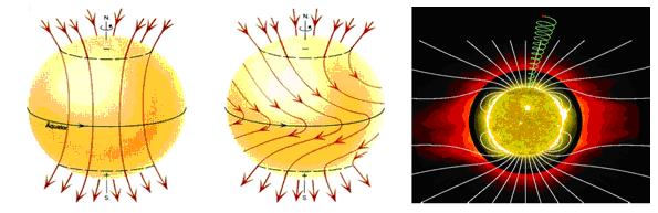
Figure 93: The strong solar magnetic field is becoming coiled toward the equator by differential rotation is strong solar magnetic field toward the equator,
with sharply defined coronal holes occuring at the poles (Source: ESA). With a magnetic dipole (like the Earth), the solar magnetic field can be compared only in a solar activity
minimum, see figure right (source: http://soi.stanford.edu/results/SolPhys200/Poletto/uvcs_spiral.jpg).
In the illustration of the Stanford University an in a magnetic field accelerated particle is shown. These particles form the solar wind and are accelerated in the radial direction away from
the sun. Because of the Lorentz force, the particles have to follow the field lines of the interplanetary magnetic field
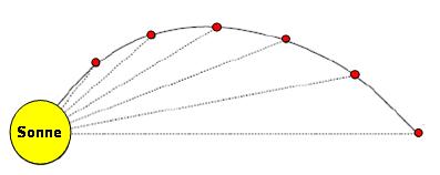
Figure 94: The radially from the solar flowing wind carries the solar magnetic field in the orbit. By the rotation arises an Archimedean spiral (curve produced by the motion of a point
at a constant speed on a beam that rotates with constant angular velocity) in which the magnetic field lines run.
This gives a resultant magnetic field in the ecliptic, that is called "Parker-spiral field" after its discoverer, the American astrophysicist Eugene N. Parker.
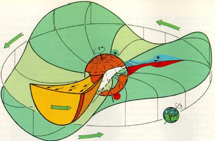
Figure 95 shows the Parker spiral in the solar minimum, source: Alfvén (1977), from Schwenn (1991). To the sun angle of 7.2 ° to the ecliptic, so does the mag. Field take up a grade
to the ecliptic. Between the magnetic north- and south half a neutral boundary layer arises, called the Heliospheric current sheet. The sudden change in the direction of the magnetic
field induces an electric current there (HCS). It separates the northern and southern hemisphere magnetic. The HCS like the IPF is subject to the solar cycle and adapts to these.
The HCS is thus a surface current which surrounds the sun more or less disc-shaped (solar minimum) and in which a reversal takes place of the horizontal magnetic field direction.
With increasing solar activity the HCS is winding more and more and takes the form of a skirt of a ballerina. In doing so their relative angle to the ecliptic moves more and more.
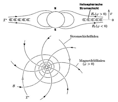
Figure 96 after Alven, 1981, shows the Heliospheric current sheet and the associated magnetic field in the meridional and in the supervision from north (magnetic south pole). The
currents flow along these logarithmic spirals (Archimedean spirals), which are perpendicular to the magnetic field lines. Adapted from "The physics of near-Earth space," Prof.
Gerd W. Prölss, University of Bonn.
The Heliospheric current sheet rotates with the sun, and an orbit takes close to 4 weeks. In this time frame, the earth is over and once again under the HCS. As the Earth in 365 days
moves around the sun once, she is repeatedly alternating in the area of south and north facing magnetic fields of the Sun, where the sun crosses each time the Heliospheric current sheet
and the Earth's atmosphere is exposed to magnetic currents in the sum of 25,000 Ampere.
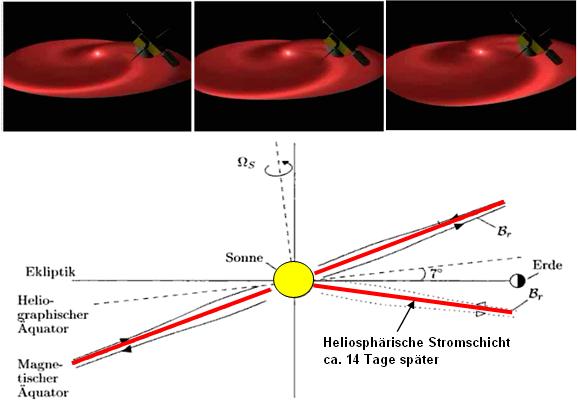
Figures 97, above (Source: NASA), show how the HCS rotates with the solar rotation and the figure below (source: Prof. Gerd W. Prölss) shows the location of the HCS and the
sun-equator and with it the position of the Earth once above and once under the HCS.
Since the position of the HCS, as already mentioned, changes with the solar activity also, a complex picture of polarity and potential crossings of the Earth to the HCS and IPF arises.
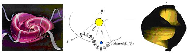
Figure 98: Left the Parker spiral is seen, that reflects the HCS. It's good to be seen that the HCS is no plane but looks like a flying ballerina skirt.
Right the HCS can be seen during the solar maximum in March 2000, when on the basis of strong magnetic activity, a second pole formed.
The HCS has more twists and assumed the shape of a snail shell (figures, source: NASA).
In the middle is shown the bending of the azimuthal component of the HCS at the height of the earth's orbit, which creates additional magnetic sectors Source: Prof. Gerd W. Prölss.
Thus the earth passes the HCS irregularly, depending on the solar rotation and magnetic activity of the sun and the solar wind, which drives the HCS in the space.
The following figure provides a spatial impression of the changing shape of the HCS during a solar rotation. It shows the HCS projected on the solar surface and thus presented in section.
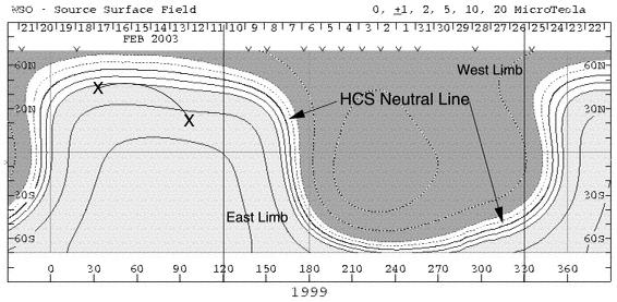
Figure 99 shows the Heliospheric current sheet in section, during a solar rotation after Hoeksema & Scherrer, 1996 (Source: wso.stanford.edu / synsource.html).
Its spatial wave character can be seen well, which spreads accordingly in the solar system and which the Earth crosses in its orbit around the sun.
Using spacecraft measurements results a disordered temporal polarity- respectively meeting pattern of the earth to the interplanetary field and to the Helio spheric current sheet.
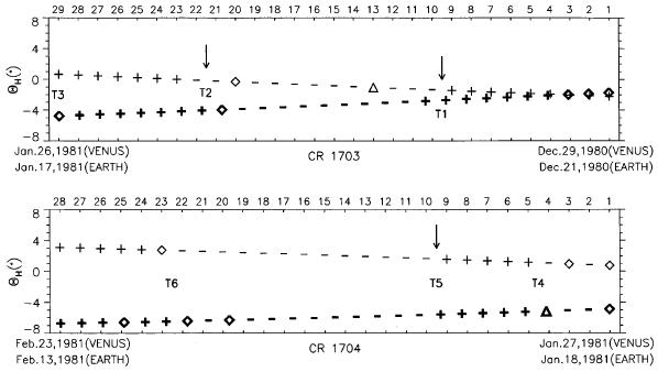
Figure 100 shows the polarities of the interplanetary field for Venus (upper series) and the Earth during the solar rotation 1703 and 1704 (CR stands for Carrington rotation). The data for
Venus derived from Pioneer Venus Observer (PVO), source:. Ma et al, "Heliospheric current sheet Inclinations at Venus and Earth ', Ann. Geophysicae 17, 642-649 (1999).
As a reference point, the angle for solar latitude is used, so the position of the sun (?H = heliographic latitude). From such comparing measurements the spatial
appearance of Helio spheric current sheet can be determined. They also show, however, when the Earth (or Venus) passed the HCS. This happens on each pole round, since the
HCS separates both pole halfes from each other.
From the data series above can be seen that the earth within a few days several times passed the Heliospheric current sheet, or stayed on this. With an active to the earth atmosphere of
about 25,000 amperes per hemisphere it can be assumed that these processes are not without influence on our immediate weather patterns. As there is a coupling between the
magnetosphere and the ionosphere of the Earth's, so is there also a coupling between the magnetosphere and the charged particles in the Stratos- and troposphere.
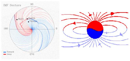
Figure 101: The field lines of the interplanetary magnetic field pointing in its course once away from the sun (away, positive polarity) and once toward the sun (toward negative polarity, above).
Correspondingly, the polarity of the interplanetary magnetic field aligns into a north and south pole component, right. Between them is the HCS. Figure 101 left shows schematically the helical
magnetic field, divided into four sectors.
Figure 101 shows that the Earth passes several times the boundary layer and thus the HCS within a short time. The HCS is subject to constant change, whereat there can only be two
sectors during a solar rotation (quiet sun). A change from positive (the two top sectors in the picture) to negative (the two lower sectors) and then back again. Or 4 sectors, as shown in the
picture. A change from 1Plus to 1Minus, back again but to 2Plus, then to 2Minus and finally back to the first sector.
In the ACE charts (ACE Advanced Composition Explorer satellite), this is measured in the phi-charts. Magnetic storms on Earth are particularly strong during an HCS crossing.
This can be an indicator that there are strong correlations between the HCS and the magnetosphere of the earth. Through their coupling to the charged particles in the underlying layers
of the atmosphere in turn directly influences of the HCS on the Stratos and the troposphere, which in turn can not be without influence on the weather.
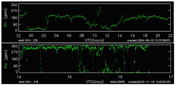
Figure 102: The green curve phi shows the HCS for one day on 22 August 2004 (Solar Cycle 23) and in the period from Nov 14 - Nov 16, 2010 (24th solar cycle). A change of
polarity (angle phi) occurs when a change between 180 ° and 360 ° respectively 0 ° or vice versa takes place. For interpretation of the trace is to be noted that the curve must be constant
for a few days before and after a change. The Stanford University (http://wso.stanford.edu/SB/SB2.html) made thereon the following condition (+ + + +: - - - -). A passage through the
HCS is in some cases a whole day. Shortly before, during and after an HCS passage solar events cause particularly strong interactions with the Earth's magnetic field!
Since Svensmark it is known and confirmed by CERN that charged aerosol particles, wich increasingly generated by cosmic rays, are up to 10 times as effective in the binding of
raindrops then uncharged. With each pass through the HCS a force component acts by the current flow on the charged particles in the tropo-and stratosphere (magnetosphere coupling to the charged particles in the
troposphere and Stratos), that changes the distribution of the charged aerosol particles. It can be assumed that there will be local concentrations, as
well as dilutions, which can not remain without direct influence on the weather patterns in the atmosphere.
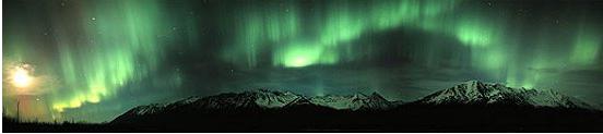
Figure 103: Atmospheric effects such as the Northern Lights (Alaska Knik Valley during the strong geomagnetic storm on 08 April 2003, NASA) are only the visible effects of
solar influences on the Earth's atmosphere. These influences are, as portrayed, far more complex and important. The solar wind stimulates in the ionosphere O2 molecules, which
emit this energy in the wavelength range of the green light again.
With the above considerations, it was assumed that the HCS in a cross-section, so in its size, is homogeneous - same magnitude as uniform direction. Of these, however, can
not be assumed, since both the solar wind, which carries the HCS, as well as the magnetic activity of the sun, which determines their strength, are not homogeneous. The
magnetic activity of the sun then imprints their pattern in the HCS. Their structures form the interplanetary medium and contribute to its dynamics.
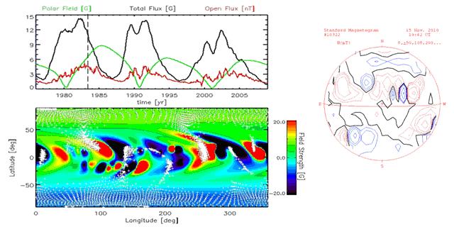
Figure 104 above shows total and open flux of the IPF during solar cycles 21 - 23, and the polar field of the sun. Below the strength of the solar magnetic field as a snapshot in
1984 (dashed line in the figure above). The open flux is the interplanetary magnetic field (its field strength), the total flux, the solar magnetic field and the polar field, the polar
magnetic field of the sun, source: (http://www.mps.mpg.de/projects/solar-mhd/research_new.html). The temporal and spatial inhomogeneities of the solar magnetic field effect that
their continuation in the interplanetary space, the IPF, as well as the boundary layer, the HCS are also inhomogeneous. The right figure shows the magnetogram of the sun for a certain
time (Nov 15, 2010, 19:42 UT), Source: WSO, Stanford University. The there to be seen and constantly changing magnetic field pattern of the sun is carried through the solar wind in
interplanetary space and thus in the Heliospheric current sheet.
Furthermore, the the solar wind and its related IPF is not only of one polarized particle type, but from both. Of positively charged protons (hydrogen atoms without an electron),
respectively ?-particles (helium nuclei, 5%) and of negatively charged electrons. Both particle-classes cause power flows which are superimposed with the solar wind according to their
distribution and influence the HCS according to their distribution patterns. In addition, the solar wind expands at supersonic speed (the prevailing speed of sound in the plasma) causing turbulence in the layer.
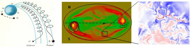
Figure 105 left shows the different deflection of positively and negatively charged particles to magnetic field lines. The figure in the center shows a section through the HCS.
The colors indicate the possible variations of the magnetic current. The thickness is more than 10,000 km. The figure on the right to show as comparison, as at small scales, the
magnetic turbulence reflect in the HCS and cause a complex pattern of magnetic current flow in the HCS.
With each pass of the Earth's atmosphere by the HCS, the atmosphere is exposed to uneven force components exerted by the inhomogeneous magnetic power of the HCS on the
magnetosphere and its coupling to the charged particles in the atmosphere. It is assumed that local accumulations as well as thinning of electrical charged aerosol particles occurs,
which is not without implications to the condensation and with that cloud cover and thus on the weather. It is known that shortly before, during and shortly after an HCS passage solar
events particularly strong act alternately with the magnetic field.
Interplanetary magnetic field (IPF)
The interplanetary magnetic field, which is designated for measurements as an open flux and is expressed in nano Tesla, is originated from the solar magnetic field, which
propagates in interplanetary space, so the space that is not determined by the planets. It works throughout the heliosphere and extends to the limits of the solar system, to the heliopause,
which is about 22.5 billion kilometers away from the sun.
In the area of the interplanetary magnetic field, a large part of the charged particles of cosmic radiation is deflected. The interplanetary magnetic field is thus a protection of the planet
from the bombardment of high energy cosmic rays.
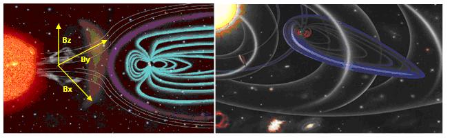
Figure 106 left shows the effects of IPF on the earth's magnetic field. The IPF can be broken down into three coordinates in space, where two are located in the ecliptic, and one (Bz)
perpendicular to it. The change of this component is particularly interesting because it runs parallel to the Earth's magnetic field and interacts with this so specially. Figure 106 on the
right shows how the field lines spread out in space of the IPF.
As already noted in the HCS, the IPF is an integral part of the solar wind and is by this spread out into space in the form of Parker spirals (quiet sun).
Solar wind and IPF are directly related to solar activity, whereat the solar wind is divided into two components, the fast solar wind with particle velocities 500-800 km/s, from coronal
holes and therefore receiving a large acceleration and the slow solar wind with particle velocities 250-400 km/s, which is chiefly from the Streamer Belt (named after photographs during an eclipse)
of the corona. The solar wind density near the Earth is 3 x 10^6 - 1 x 10^7 particles/m3. While the strength of the IPF (open flux) is specified in nano Tesla, the solar wind flux is specified
in particles/m^3 and the strength of the solar wind in nano-Pascal. The magnetic field in the active regions of the Sun is called non-axis-symmetric open flow and the magnetic field
from the polar regions, axis symmetrical open flow, because this field is symmetrical to the axis of the sun (figure below ).
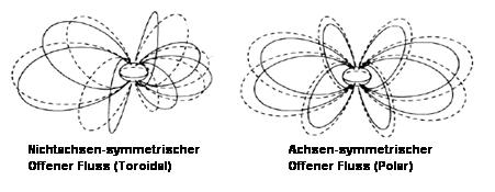
Now the question may arise why the solar magnetic field must be divided into components at all because on earth the entire magnetic field of the sun is effective. The special
position of the Bz component of the IPF was already mentioned. For the effect of cosmic radiation on the earth, however, is significant that in the orbital plane, in which the planets move,
expanding solar magnetic field. This is the Nonaxisymmetric Open Flux. The solar wind strength in turn depends on the both (polar and toroidal), wherein the
particles at a higher speed are from the Polar field, the coronal holes. The activity of the polar field to the total open flux is reversed, and disappears in the solar maximum.
From the solar wind speed can therefore only partly concluded on the activity of the sun.
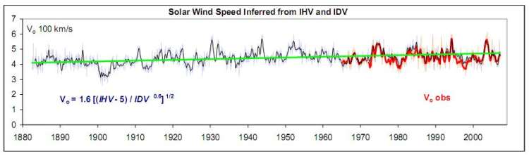
Figure 107 (Source: www.leif.org/research/files.htm) shows the 27-day averages of solar wind speed at 100 km/s from 1880 to 2009, according to Leif Svalgaard. Blue, from
IHV (Inter-Hour Variability index) and IDV (International Diurnal variability) reconstructed; red are directly measured values. In the solar wind speed the basic solar cycles are
visible, but from this alone any conclusions on global temperatures are not possible. This requires additional parameters.
According to data from NASA, the solar wind in the first decade of the 21st Century dramatically decreased, which, as already shown several times, leading back to the current weak
solar activity. So figure 108 left shows the strength of the solar wind and Figure 108 right as with him, or more precisely, the solar activity (as known, the solar wind is related to her),
the global temperatures vary.
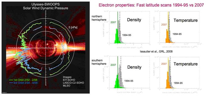
Figure 108: Left using the Ulysses data, the strength of the solar wind (the product of particle velocity and the corona temperature) in the period from 02/92 - 02/98 (green) and from 02/04
- 08/08 (blue) is represented as an area chart. Since the coronal temperature in direct degree reflects the magnetic activity of the sun - the corona is heated by this (see
reconnection and coronal) - the solar wind strength is the measure of solar activity. In the figure on the left, the two coronal holes in the North and South stand out sharply, Source:
NASA, "Solar Wind Loses Power, Hits 50-Year Low", 23.09.2008. It can clearly be seen that the sun is quiet between 2004-2008. Right is shown as a histogram, the intensity and distribution
of the solar wind, separately for the northern and southern hemisphere of the earth, and beside it, also as a histogram, the global ground temperatures. Global temperature and solar
activity are identical to the investigation of NASA.
These figures show that the declining temperatures, the way as we have seen them (not like the WMO wants to sell them to us) in recent years are due to the reduced solar activity. The
Ulysses data show that the average solar wind pressure decreased by 20%, mainly due to the lower temperature of the corona and the reduced solar wind strength
(particles/m^3). Thus, the solar wind in the same period got 13% cooler and 20% lower. According to measurements by NASA the solar magnetic field decreased by 30% during the period.
It was already mentioned that the Bz component of the IPF has a particular importance, since this component interacts the most with the Earth's magnetic field. Thus, auroras, which are
directly observable signs of strong solar activity, are the more likely the stronger the IPF and the more negative her component, the Bz is. This is related to the fact, that south (negative)
directed magnetic fields of the IPF, which run antiparallel to the magnetic field lines of the Earth's magnetic field, weaken the magnetic field of the Earth, creating thereby a
magnetic short circuit ("merge" with the field lines). The magn. shield of the earth is then punctured and charged particles can move up into lower latitudes into the deeper layers of the
atmosphere of the Earth. According to research by NASA up to 20 times more charged particles reach then into the lower layers in the atmosphere!
It is known, that the effects of the particle flows in the polar regions are the greatest, because the magnetic field lines flow out there. Therefore it is natural to investigate to what extent this
affects the local climate parameters, if it is postulated that charged atmosphere particles control the weather, and thus the temperature.
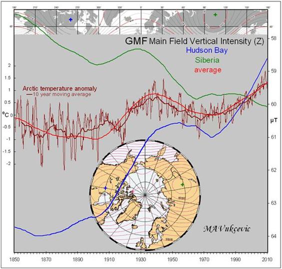
Figure 109: To see (Source: www.appinsys.com/Global Warming/EarthMagneticField.htm) are respectively the vertical (Z) component of the geomagnetic field. This is directly
related to the interplanetary magnetic field (GMF = Geo MAGNETC Field). Selected were two points opposite each other (red and green cross) and their resultant close to the
magnetic north pole (red curve). The temperature response of the arctic temperatures agrees exactly with the magnetic activity and thus coincide with the solar activity.
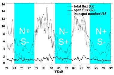
Figure 110a: For current temperature trends mostly 30-year comparisons are used, because this time window is defined as climate by definition. If the last 30 years are used, this
period falls together with the above magnetic polarity of the solar magnetic field. During this period (to 2009) twice the magnetic
North Pole was located at the geographic North Pole of the Sun. This means in the solar minimum, that the field lines are oriented antiparallel to the Earth's magnetic field.
As is known, anti-parallel alignment of the IPA field lines leads to a weakening of the geomagnetic field, which get more charged particles in the lower atmosphere. Now the solar magnetic
field is no dipole, as seen in the HCS and the earth is not constantly in the field of one polarity, especially when solar activity increases, with a quiet sun, however, the above
polarization pattern applies, and it is only for the periods in the solar minimum shown on a blue background.
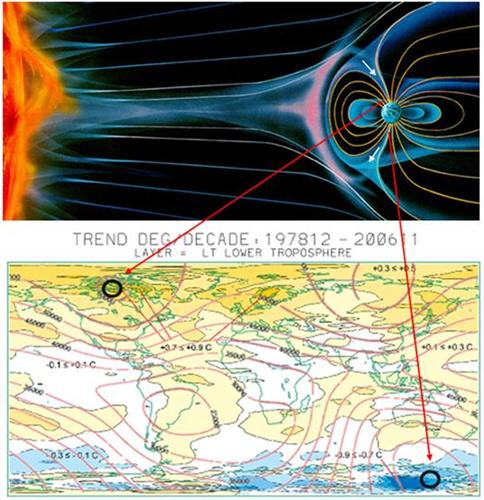
Figure 110b Source: (http://www.appinsys.com/GlobalWarming/EarthMagneticField.htm) shows simplified the interaction of IPV with the Earth's magnetic field (white arrows)
and the course of the field lines in the solar minimum, when magnetic and geographic north pole are physically together. Below are the global temperature anomalies shown in
the area for the period 12/1978 - 11/2006. At the magnetic north pole (circle), where the field lines and thus incorporate the charged particles flow in, there is a
temperature increase and at the South Pole, where the field lines leave, so no particles flow in, there is a significant decrease in temperature. Arctic-Antarctic climate swings!
The polar temperature distribution on the previous page is an indication that charged aerosol particles have a directly influence on weather and thus on the temperature.
Where the magnetic field lines and and with them ionized particleflow flow in, according to NASA (http://www.nasa.gov/mission_pages/themis/news/themis_leaky_shield.html)
a 20-fold increase of the ionized sun-particles occurs and there also is the most obvious increase in temperature. In counter-pole we see the most obvious decrease in temperature.
The finding from the figure, is also a starting point for the Seesaw between the Arctic and the Antarctic justified theoretically on short time scales.
That it comes to a compression at the poles, ie an accumulation of charged particles, is caused on the one hand, on the profile of the magnetic field lines and, second, that the auroral
region between 1000-4000 km altitude has such as an electrostatic accelerator effect on charged particles, .
Electrons and ions are due to their different electric charge thereby accelerated along the field lines in opposite directions. Measurements have shown that the acceleration takes
place in stationary horizontal layers of 10-20 km vertical thickness (source: MPS). Here, electrons are accelerated downwards and can thereby ionize molecules, and these then
carry a negative charge.
There are other documents which show that the cloud cover and thus the condensation nuclei, or aerosols, which are necessary as a precondition for the emergence of
water particles in the atmosphere, depend on the polarity of the solar field. These are the data on global cloud cover from the ISCCP (International Satellite Cloud Climatology Project).
According to Svensmark is already known that the cloud cover varies with the cosmic radiation (Figure 111). The cosmic radiation again is opposite to the solar activity and the
11-year Schwabe cycle is characterized by the fact more apparent.
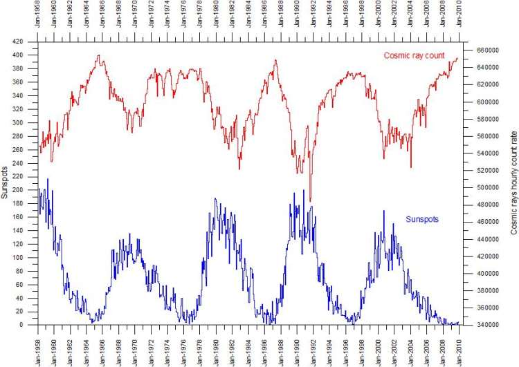
Figure 111 (http://www.climate4you.com/Sun.htm) shows the sunspot number and cosmic ray intensity (neutron monitor) from January 1958 - 06th November 2009. It is clearly
apparent that increased solar activity shields the earth from cosmic radiation. During a solar cosmic radiation more activity minimas reaches to Earth.
The physical explanation for this relationship is set forth pictorially in the following figure in the right.
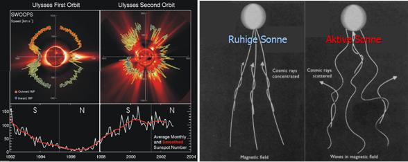
Figure 112, far left, shows the sun's magnetic field as a dipole field in the solar minimum taken from the solar probe Ulysses (SWOOPS = Solar Wind Observations
Over the Poles of the Sun). In addition, the magnetic field during the activity maximum. Right, the course of the charged particles of cosmic radiation on the magnetic field lines
of the sun are shown. At wound magnetic field lines during high solar activity, the particles are deflected and spread outward from the solar system.
That the cosmic rays runs in the counter clock to the solar activity, is primarily due to the higher amount of solar activity and further that the solar magnetic field is only in the activity
minimum a dipole field, whereas with increasing solar activity, the polarities (the incoming and outflowing magnetic field lines, award, or toward-the IMF, see HCS) get more and more
mixed and the magnetic field lines more and more wound up.
The following sections show how the previously in theory shown affect the weather and climate events.
Part 1: The sun sets the temperature response
Part 2: The sun - the amazing star
Part 3: Sunspots and their causes
Part 4a: The atmosphere of the sun: The corona
Part 4b: Heliospheric current sheet and interplanetary magnetic field
Part 5: The atmosphere of the sun: The corona
Part 6: The influence of the sun on our weather / climate
Part 7: The influence of the sun on the cloud cover beyond Svensmark
Part 8: Future Development and the temperature fluctuations
|
|
|